Empirical Bayes-ketball

How much can you learn about the three-point shooting of a player when data is limited?

Potential lottery picks Cole Anthony and Tyrese Haliburton only played 22 games before injuries cut their season short in 2020 (finishing with 141 and 124 three-point attempts respectively). Potential #1 draft pick LaMelo Ball had 80 three-point attempts in his 12 NBL games. The top high school recruit in the country James Wiseman missed his only three-point attempt in just 69 minutes at Memphis.

How do you confidently evaluate shooting performance based on such limited data?

This is especially important in a year where numerous NBA lottery picks will be selected based on so few data points.

---

Trying to find a signal in the noise with such small sample sizes is not a new problem in sports analytics. This comes up every year in the MLB after a player starts the season on a hot streak, giving hope that they will be the first person to hit .400 since Ted Williams last did in 1941. As a good Bayesian we know that a player batting over .400 after 100 at bats has a better shot than another player after only 10 at bats, but neither are likely to top .400.

One simple approach to estimate a player's end of season batting average, is to regress their current average to the mean. For example, take a weighted average of current batting average with the league average, weighting based on how far along in the season they are (or better yet regress against their career average).

This simple concept is the basis for approaches referred to as the "stabilization rate" or "padding method" (often used by @Tangotiger). You may have also heard of this in relation to a concept called "Empirical Bayes", as there is a whole series of blog posts that apply Bayes to batting averages (along with many other interesting extensions).

---

Which NBA player has had the best three-point shooting season of all time?

The easiest way to answer this question is to look at single season 3P% leaders. Note that for the sake of simplicity we will overlook shot difficulty and league-wide changes in three-point shooting trends.

rank	name	team	year	3p%	3pm	3pa
1	Jamie Feick	NJN	2000	1.000	3	3
2	Raja Bell	GOS	2010	1.000	3	3
3	Antonius Cleveland	ATL	2018	1.000	3	3
4	Beno Udrih	MEM	2014	1.000	2	2
5	Don MacLean	MIA	2001	1.000	2	2

Looks like the top seasons are all from players shooting 100% on only a few shot attempts - therefore it doesn't look like this approach is particularly informative.

As a next step, we can apply a filter to exclude seasons with <X three-point attempts (I choose an arbitrary threshold of 100 attempts below).

rank	name	team	year	3p%	3pm	3pa
1	Pau Gasol	SAN	2017	0.538	56	104
2	Kyle Korver	UTH	2010	0.536	59	110
3	Jason Kapono	MIA	2007	0.514	108	210
4	Luke Babbitt	NOP	2015	0.513	59	115
5	Kyle Korver	ATL	2015	0.492	221	449
6	Hubert Davis	DAL	2000	0.491	82	167
7	Kyle Korver	CLE	2017	0.485	97	200
8	Troy Daniels	CHA	2016	0.484	59	122
9	Fred Hoiberg	MIN	2005	0.483	70	145
10	Jason Kapono	TOR	2008	0.483	57	118

This list is more intuitive but with Pau Gasol leading the pack and Steph Curry not even on the list…we remain skeptical. This approach is also sensitive to the specific threshold chosen which adds undesirable subjectivity to the process. There must be a better way…Empirical Bayes!

Empirical Bayes methods are procedures for statistical inference in which the prior distribution is estimated from the data.

Since drob@ does a better job explaining these concepts than I ever will, I highly recommend reading his Empirical Bayes book which is a compilation of baseball themed blog posts on the topic. He does an excellent job explaining concepts using practical examples and even includes sample code to follow along.

The only thing missing is Python specific code (thanks stackoverflow!) - which is why I've included a code snippet to aid others in performing their own Empirical Bayes! This code assumes a beta-binomial distribution, which is great for sports analytics because it can be applied to any "success/attempt statistic".

from scipy.stats import betabinom

from scipy.optimize import minimize


def betabinom_func(params, *args):

    a, b = params[0], params[1]

    k = args[0] # hits

    n = args[1] # at_bats

    return -np.sum(betabinom.logpmf(k, n, a, b))


def solve_a_b(hits, at_bats, max_iter=250):

    result = minimize(betabinom_func, x0=[1, 10],

              args=(hits, at_bats), bounds=((0, None), (0, None)),

              method='L-BFGS-B', options={'disp': True, 'maxiter': max_iter})

    a, b = result.x[0], result.x[1]

    return a, b


# Sanity check your data to ensure hits <= at_bats, at_bats > 0, and both are type int

def estimate_eb(hits, at_bats):

    a, b = solve_a_b(hits, at_bats)

    return ((hits+a) / (at_bats+a+b))


df['3p%_eb'] = estimate_eb(df['3pm'], df['3pa'])

The results look much better after applying Empirical Bayes - many great shooters and multiple Curry sightings!

rank	name	team	year	3p% (eb)	3p%	3pm	3pa
1	Kyle Korver	ATL	2015	0.446	0.492	221	449
2	Stephen Curry	GOS	2016	0.433	0.454	402	886
3	J.J. Redick	LAC	2016	0.433	0.475	200	421
4	Joe Johnson	PHX	2005	0.431	0.478	177	370
5	Jason Kapono	MIA	2007	0.431	0.514	108	210
6	Glen Rice	CHA	1997	0.431	0.47	207	440
7	Joe Harris	BRK	2019	0.429	0.474	183	386
8	Kyle Korver	ATL	2014	0.428	0.472	185	392
9	Steve Nash	PHX	2008	0.426	0.47	179	381
10	Stephen Curry	GOS	2013	0.426	0.453	272	600

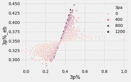
It is also interesting to look at how strongly results are regressed towards the mean depending on how many attempts a player has (explore the drop-down for the same approach applied to other stats!).

3P% 2P% FG% FT% AST% BLK% DRB% ORB% STL% PF% TOV% USG% EFG% FTR 3PAR

I included the optimal alpha/beta values in a table below so you can regress statistics on your own¹. I'll leave it to the reader to compare these results with other techniques like NBA stabilization rates (recent work by @kmedved).

stat	success	attempt	alpha	beta	avg
3p%	3pm	3pa	73.2	137.3	0.348
2p%	2pm	2pa	54.9	60.7	0.475
fg%	fgm	fga	44.4	55.2	0.446
ft%	ftm	fta	15.5	5.5	0.736
ast%	ast	ast_opp	2.1	13.8	13.5
blk%	blk	opp_2p_fga	0.7	20.7	3.1
drb%	drb	drb_opp	6.0	35.4	14.5
orb%	orb	orb_opp	2.0	33.0	5.7
stl%	stl	poss	8.4	508.0	1.6
pf%	pf	poss	8.5	159.8	5.0
tov%	tov	poss	13.3	83.6	13.8
usg%	usg_num	poss	12.0	52.2	18.7
efg%	efg_num	fga	60.4	63.8	0.486
ftr2	fta	fga	2.8	6.7	0.292
3par	3pa	fga	0.5	1.9	0.214

Note that these numbers are based on NBA data dating back to the 1996-97 season. The game is continually evolving, which means different time periods can change results slightly. With additional complexity it is possible to enhance the approach by calculating different values for each season or decade.

---

When dealing with limited data (as is often the case in sports analytics), Empirical Bayes is a powerful tool. By objectively regressing towards the mean, we can avoid outlier data points and more accurately evaluate small sample performances.

In my next post, I will discuss a related topic of "hierarchical modeling" and look at some specific examples from the 2020 draft class.