NFL Big Data Bowl - PassNet

After submitting an entry to the 2021 Big Data Bowl in which I evaluated new Next Gen Stats for pass defense (honorable mention! again…), I decided to play around with an entirely different idea. This work was inspired by the 2020 Big Data Bowl winning solution which used Convolutional Neural Networks (CNN) to predict expected rush yards at the time of handoff.

Goal

My objective was to build a CNN model using NFL tracking data to predict expected pass play outcomes at every frame of a play (i.e. every tenth of a second).

Not only would it be fun to see how the expected pass outcome changes in real-time as plays develop (analytics broadcast anyone!?) - I have an even cooler application that I'll share soon!

Evaluating pass play outcomes in real-time

In the example below we can see how various outcomes (i.e. EPA, Success Rate, TD Probability) change in real-time as the play progresses.

In this particular example, a perfect Patrick Mahomes throw turns a negative expectation play (at time of throw) into an 89-yard touchdown. After the receiver catches the throw in stride and the defender falls down, the TD probability jumps from near zero to almost certain in a matter of a few tenths of a second.

Below is an actual video of the play:

If you don't care about nitty gritty model details, skip down to see more sample plays.

Approach

Similar to the 2020 Big Data Bowl winning solution for "expected rush yards", I found that a highly predictive CNN model can be built using only the location and speed of players (and football) at a single instant of the play. The basic intuition behind my approach is that there are two groups of players: (1) offensive players - who are trying to advance the football downfield via a pass and (2) defensive players - who are trying to interact with offensive players to prevent a successful pass.

The structure of the model follows this same intuition - one convolution for offensive players using location and speed relative to the football and a second convolution for defensive players relative to each offensive player.

Data

To train the CNN models I used the 2021 Big Data Bowl dataset which includes NFL tracking data across all 19,239 pass plays from the 2018 regular season. With the typical passing play lasting ~5.5 seconds and tracking data existing for each tenth of a second, there are on average around 55 "frames" of movement data per play. On each play the tracking data captures player movement data for all non-lineman offensive players (typically 6) and defensive players (typically 7+).

I filtered out pre-snap data and various small-sample edge cases (i.e. offensive players < 6, defensive players < 7, no football tracking data). I also excluded plays with a penalty to avoid noise being fed into the model when player movement doesn't necessarily align with pass play outcome (the EPA outcome in particular).

Data processing

Tracking data was normalized from left to right (in terms of field direction). To improve CNN performance, each play was replicated with an inverted Y axis in training data (i.e. augmentation) under the assumption that mirrored plays will have identical outcomes. Data for model features was standardized.

To deal with variability in terms of number of defensive players with tracking data across plays (i.e. most commonly there is data for 7 defensive players, but it will vary anywhere from 7 to 11 depending on the play), I filtered to the 7 players furthest from the original line of scrimmage at the time of pass (or sack) as I assume those players are most responsible for pass coverage. I made this decision (instead of populating with zeros for example) to avoid introducing sampling bias if plays with tracking data for >7 defensive players happened to correlate with play outcome.

Models

1. EPA - Expected points added
2. SR - Expected offensive success rate (as determined by whether a play had positive EPA)
3. COMP - Expected probability of pass completion
4. TD - Expected probability of touchdown
5. INT - Expected probability of interception

Model Structure

The structure of my CNN follows the success from the 2020 Big Data Bowl winning solution (which someone kindly replicated here). Each "image" (i.e. row of data) fed to the CNN represents a single "frame" from a given passing play. In total, the models were trained on ~2 million unique "images". Each image is transformed into the following vector features (6 offensive players x 7 defensive players x N features):

• off x,y - football x,y
• off sx,sy - football sx,sy
• off sx,sy
• def x,y - off x,y
• def sx,sy - off sx,sy

While not required to have a solid model, I also explored adding the following features to improve performance, particularly for the EPA/SR models where it is useful to have more situational context:

• off x - los x (relative to line of scrimmage)
• off x - first x (relative to first down marker)
• off x (relative to end zone)
• down of play (1,2,3,4)

Training

Models were trained on week's 1->16 with week 17 used as hold out data (for evaluation and analysis). Bagging was used to improve model performance with predictions averaged.

Evaluation

As noted, evaluation metrics are based on week 17 holdout data.

Model	Correlation	MAE	AUC	Accuracy
EPA	0.538	0.97	n/a	n/a
SR	0.488	n/a	0.77	0.682
COMP	0.533	n/a	0.814	0.694
TD	0.476	n/a	0.897	0.914
INT	0.386	n/a	0.79	0.94

The INT model could be better (interceptions have a lot of randomness to them) but otherwise performance is not bad!

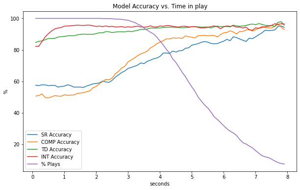
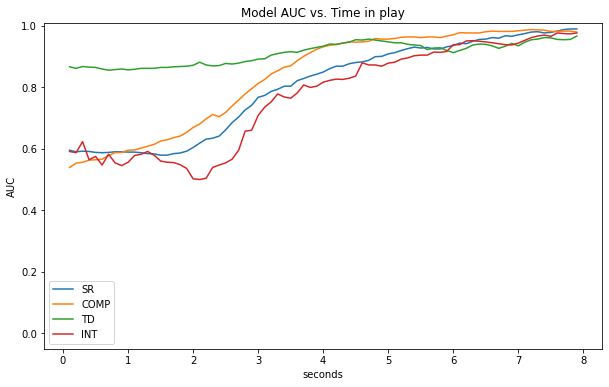
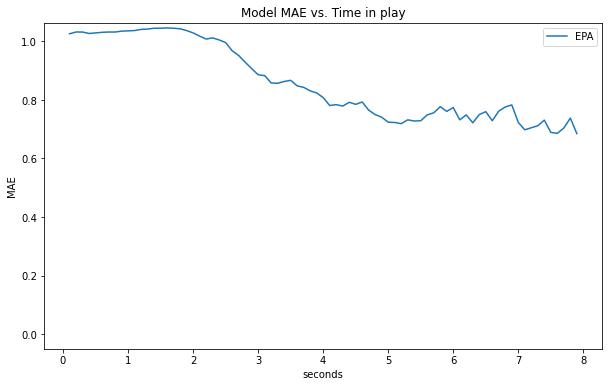
Note that these statistics are equally weighting each frame, which means plays that last longer represent a higher proportion of the total data. We can ensure longer plays aren't biasing our results by looking at performance at specific events (e.g. at snap, at time of throw) or across frame numbers (i.e. frame 1, frame 2, etc.) - the latter is done below.

As a play progress, we expect that the play outcome becomes more obvious (i.e. towards the end of a play, the ball location and closest player is very telling of the outcome). As expected, we can see model accuracy improves as time advances.

Highlighted Plays

Below are various top plays from Week 17, which showcase how expected outcomes change in real-time as a play evolves.

Russ to Lockett Pass

In this play Russell Wilson steps outside of the pocket and throws a 37-yard dime to Lockett. After the ball is thrown the real-time EPA increases as the intended WR becomes known. Interestingly, the EPA drops for a few frames as the pass is going over the head of the Cardinals defender (#41) which is because the model doesn't know how high in the air the ball is (adding z-axis football coordinates can improve!). The plays ends with a predicted EPA of ~2.5 which is close to the actual EPA of 1.8 (watch the video).

D.J. Moore Great Catch

On this 3rd down play we can see D.J. Moore is well covered by Marshon Lattimore all throughout, which translated to a low completion probability until the very end when Moore makes an amazing catch (watch the video).

Big Ben Interception

After Ben throws the ball into coverage we can see the interception probability quickly increase and then spike up after the ball is caught. After the interception starts to be returned for a TD, the model sees that the football and most players are moving towards the Bengals endzone, which bumps the interception probability up even more (watch the video).

Baker Pass Under Pressure

Baker buys just enough time for Higgins to free up and then makes a strong throw under pressure to flip the success rate probability in the Brown's favor (watch the video).

Follow me on Twitter and I might share some more interesting plays.